Software

ade

Asynchronous Differential Evolution, with efficient multiprocessing

Differential Evolution (DE) is a type of genetic algorithm that works especially well for optimizing combinations of real-valued variables. The ade Python package does simple and smart population initialization, informative progress reporting, adaptation of the vector differential scaling factor F based on how much each generation is improving, and automatic termination after a reasonable level of convergence to the best solution.

But most significantly, ade performs Differential Evolution asynchronously. When running on a multicore CPU or cluster, ade can get the DE processing done several times faster than standard single-threaded DE. It does this without departing in any way from the numeric operations performed by the classic Storn and Price algorithm, using either a randomly chosen or best candidate scheme.

You get a substantial multiprocessing speed-up and the well-understood, time-tested behavior of the classic DE/​rand/1/bin or DE/​best/1/bin algorithm. (You can pick which one to use.) The very same target¹ and base² selection, mutation,³ scaling, and crossover⁴ are done for a sequence of targets in the population, just like you’re used to. The underlying numeric recipe is not altered at all, but everything runs a lot faster.

How is this possible? The answer is found in asynchronous processing and the deferred lock concurrency mechanism provided by the Twisted framework.

Lots of Lock

The magic happens in the challenge method of the DifferentialEvolution object. Before considering what’s different about this, let’s consider what’s the same as usual. Here’s a simplified version of the method, omitting some if-then blocks that can be disregarded while the algorithm is running:

@defer.inlineCallbacks
def challenge(self, kt, kb):
    k0, k1 = self.p.sample(2, kt, kb)
    # Await legit values for all individuals used here
    yield self.p.lock(kt, kb, k0, k1)
    iTarget, iBase, i0, i1 = self.p.individuals(kt, kb, k0, k1)
    # All but the target can be released right away,
    # because we are only using their local values here
    # and don't care if someone else changes them at this
    # point. The target can't be released yet because its
    # value might change and someone waiting on its result
    # will need the accurate one
    self.p.release(kb, k0, k1)
    # Do the mutation and crossover with unbounded values
    iChallenger = iBase + (i0 - i1) * self.fm.get()
    self.crossover(iTarget, iChallenger)
    # Continue with Pr(values) / Pr(midpoints)
    self.p.limit(iChallenger)
    if self.p.pm.passesConstraints(iChallenger.values):
        # Now the hard part: Evaluate fitness of the challenger
        yield iChallenger.evaluate()
        if iChallenger < iTarget:
            # The challenger won the tournament, replace
            # the target
            self.p[kt] = iChallenger
    # Now that the individual at the target index has been
    # determined, we can finally release the lock for that index
    self.p.release(kt)

The DifferentialEvolution.challenge method challenges a target (“candidate,” or “parent”) individual at an index kt in the population with a challenger individual. These “individuals” are instances of the Individual class. Each instance mostly acts like a sequence of float values–a chunk of digital DNA–to feed to your evaluation (fitness) function. It has an evaluate method that you run to obtain a sum-of-squared error result of that function, which gets stored in the individual’s SSE attribute. It also has some methods that make comparisons with other individuals easier.

The DE algorithm runs the challenge method for each individual in the population, considering that individual the target of a possible replacement. It creates a challenger in a multi-step process. First, it computes the vector sum of a base individual (at index kb) and a scaled vector difference⁵ between two randomly chosen other individuals that are distinct from each other and both the target and base individuals. Then it does a crossover operation between this intermediate result (I call it a mutant) and the target, randomly selecting each real-valued sequence item from either the mutant or the target. Here’s what the crossover method looks like:

def crossover(self, parent, mutant):
    j = random.randint(0, self.p.Nd-1)
    for k in range(self.p.Nd):
        if k == j:
            # The mutant gets to keep at least this one value
            continue
        if self.CR < random.uniform(0, 1.0):
            # CR is probability of the mutant's value being
            # used. Only if U[0,1] random variate is bigger (as it
            # seldom will be with typical CR ~ 0.9), is the mutant's
            # value discarded and the parent's used.
            mutant[k] = parent[k]

The mutant is modified in place. Note that, with typical CR values closer to 1.0 than 0.5, it’s more likely that a given sequence item will be from the mutant than from the target. That makes sense, since we are challenging the target with something different, and we’d just be wasting time if we made the something different barely different at all.

So far, all of this is conventional Differential Evolution. If the base individual is randomly chosen (but never the same as the target), then it is referred to as DE/​rand/1/bin. If the base is always the best individual in the population (with the lowest SSE), then you are running DE/​best/1/bin.

In either case, two other individuals (never the same as the target or base) are randomly chosen from the population to compute a scaled vector difference from. The challenge method references these individuals from a Population object via integer indices. The target’s index in the population is kt, the base’s index is kb, and the two randomly chosen other individuals have indices k0 and k1. The sampling of k0 and k1 is shown in FIG. 1. The population members (individuals) are shown in the upper array p.⁶

Critically, there’s something else going on that’s also shown in FIG. 1. Each individual has its own concurrency lock, in the lower array d.

FIG. 1: Begin the challenge by acquiring concurrency locks.

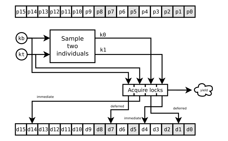
Each lock is an instance of the Twisted⁷ framework’s DeferredLock. When you try to acquire one of those, it returns a Deferred object that fires when, and only when, the lock is yours. The challenge method acquires all the locks for all four individuals involved in the challenge and yields a Deferred that fires when all four locks have been acquired. That happens, incidentally, with a call to the Population object’s lock method:

def lock(self, *indices):
    """
    Obtains the locks for individuals at the specified indices,
    submits a request to acquire them, and returns a `Deferred`
    that fires when all of them have been acquired.
    """
    dList = []
    for k in indices:
        if indices.count(k) > 1:
            raise ValueError(
                "Requesting the same lock twice will result in deadlock!")
        dList.append(self.dLocks[k].acquire())
    return defer.DeferredList(dList).addErrback(oops)

Now, the example of FIG. 1 is a challenge of the individual at p14. That’s the target. The individual at p7 is the base, and the individuals at p1 and p4 were selected for the vector subtraction operation. We need valid digital DNA for all four of those individuals before we can proceed. But when our challenge starts, the individuals at p8, p7, p5, p2, p1, and p0 are busy getting evaluated for other challenges, as indicated by the grey boxes. We can have the locks d14 and d4 right away, but we need to wait for the locks d7 and d1. So we yield the Deferred until we can have it all.⁸

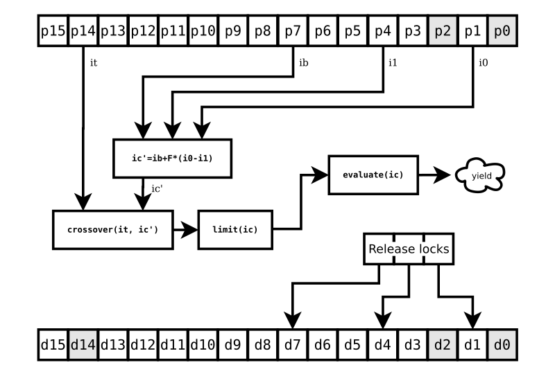
Once that Deferred fires, we resume the challenge method at FIG. 2. Note that the individuals at p2 and p0 are still not ready. But we don’t care about that, because our particular challenge is completely unaffected by them.

We release the locks d7, d4, and d1 as soon as we’ve retrieved copies ib, i1, and i0 of the individuals at p7, p4, and p1. Once we have those copies, we don’t care how the population updates at those positions. Entirely new individuals could occupy those slots right away for all we care. We have what we need for the challenge to the individual at p14.

We proceed with the conventional DE steps for challenging the target individual:

That last step is what takes a while; otherwise you wouldn’t be bothering with trying to speed up your DE heuristics. And so your fitness function must not block, but rather return a Deferred that fires with the SSE when it’s available. Look at the two examples included with ade to see how you might implement a Twisted-friendly, asynchronous evaluation function.

FIG. 2: Do the DE stuff, releasing what locks we can.

This is the key to the performance gain that ade gives you: It goes through each target of the population asynchronously. It doesn’t wait for one target to finish being challenged before starting a challenge on the next. So there are other challenges going on when we start our example challenge of the individual at p14. But we can only proceed with a challenge once all the individuals involved are ready.

FIG. 3 shows what happens when your CPU-burning evaluation function finally gets done. A tournament (really, just an if statement comparing the two individuals) determines if the challenger gets to take the place of the target. And now, only now, we can release our last lock, d14.

FIG. 3: The challenger wins; replace target and release its lock.

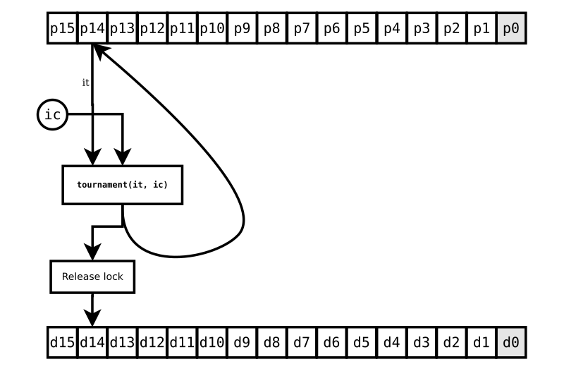
The individual at p0 still isn’t ready, but who cares? It means nothing to this challenge. But imagine other challenges going on as all this happens. Say there’s one challenging the next individual in the population, at p13, that uses our target individual (at p14) as its base. It can’t proceed until our challenge is done. And, if it’s so unfortunate as to have chosen the individual at p0 as its i0 or i1, it might be waiting a while.

Fortunately, Differential Evolution is typically run with dozens or even hundreds of population members, many more times than the four or eight CPU cores you have available.⁹ So the asynchronous processing will usually find a target it can work on that does have four individuals all ready to be accessed, and thus without disturbing the classic numeric recipe of DE. When you watch the progress of each generation, you’ll see it start out fast as the CPU cores finds lots of challenges to proceed with and then slow down as the unfortunate challenges that depend on slow results are all that’s left to do. Even so–as long as your evaluation function is dispatched to an idle CPU core and doesn’t block–ade will typically speed up your Differential Evolution by a factor of several times.

Examples

The ade package comes with two example Python scripts. You can extract the scripts and their support files to a subdirectory ade-examples of your home directory by typing the following in a shell:

You will see something like this:

The Goldstein-Price Test Function

The Goldstein-Price test function

Do a cd to the newly created ~/ade-examples directory and compile goldstein-price.c there using gcc:

Then you can run the example script:

You will see stuff fly by on the console that show progress of the Differential Evolution algorithm. This little compiled test function runs so fast that you can barely tell there’s anything significant going on. Take a look at goldstein-price.log to see what the result looks like after running on my eight-core CPU; it takes about 0.7 seconds to converge and stop trying any more DE generations.

The population is fairly small (40 individuals) in this example, so there’s not as much benefit from the asynchronous multi-processing.¹⁰ But it still runs about twice as fast with four CPU cores as it does with just one. Try changing the value of N in the Solver class of ~/ade-examples/​goldstein-price.py to see how much difference the number of parallel processes makes on your CPU.

One important thing to observe about this example is how it does its evaluation function in an asynchronous multiprocessing-friendly fashion. The key to that is found in the cmd and outReceived methods of the ExecProtocol class, which implements a Twisted process protocol:

@defer.inlineCallbacks
def cmd(self, *args):
    """
    Sends function arguments to the executable via stdin, returning
    a C{Deferred} that fires with the result received via
    stdout, with numeric conversions.
    """
    yield self.lock.acquire()
    self.transport.write(" ".join([str(x) for x in args]) + '\n')
    yield self.lock.acquire()
    self.lock.release()
    defer.returnValue(float(self.response))

def outReceived(self, data):
    """
    Processes a line of response data from the executable.
    """
    data = data.replace('\r', '').strip('\n')
    if not data or not self.lock.locked:
        return
    self.response = data
    self.lock.release()

Deferred locks again! In this case, a lock is acquired when the x and y variables are sent to the compiled goldstein-price function via STDIN and released when a result is received via STDOUT. The cmd method yields the Deferred object from its attempt to acquire the lock, and so it plays nice with the Twisted reactor and lets ade do its asynchronous thing.

The ExecProtocol is used by a Runner object, which spawns an instance of the goldstein-price executable you compiled. One instance of MultiRunner manages a pool of Runner instances; as a callable object, it serves as the evaluation function for the DE algorithm.¹¹ Each call to the MultiRunner object acquires a (deferred) instance of Runner from a DeferredQueue and calls it (when available) to obtain the Goldstein-Price function’s value for a given pair of x and y values. Take a look at the goldstein-price.py script to better understand how all of these pieces fit together in just a couple hundred lines of object-oriented Python code.

Nonlinear Curve Fitting

Our second example fits a nonlinear curve to filtered voltage and temperature observations. It is pure Python (nothing compiled), and chews on a lot of data points, and so it takes a while to converge to a solution even with multiple CPU cores cranking away. On my eight-core CPU running at about 4 GHz, ade required just over 31 minutes to reach the solution shown in FIG. 4 and stop. (It took five times as long to reach a comparable solution and stop on another run I did that was limited to using just one core.)

FIG. 4: Nonlinear curve fit found after 70 DE generations

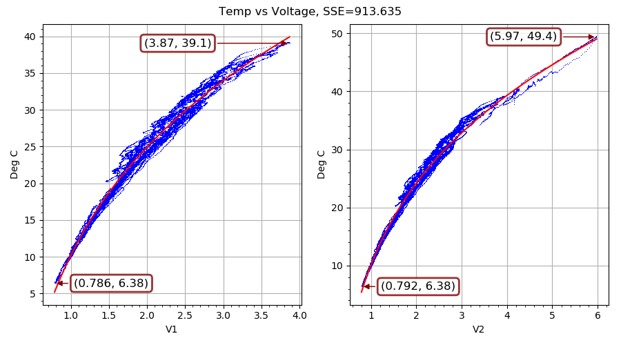
This example resulted from a slightly over-designed solution to an actual engineering problem. I had commisioned an outdoor equipment shed that gets quite hot with the electrical stuff operating inside. I wanted to run a ventilation fan when doing so would cool things off, and only then. What I had handy for measuring inside and outside temperatures was some thermistors and a dual-input USB-connected voltage measuring device made by a cool little Swiss company called YoctoPuce. On a temporary basis, I also had access to a precision temperature measuring device.

On each of the two inputs of the voltage measuring device (a Yocto-0-10V-Rx), I connected a voltage divider with a 100K NTC thermistor in the upper leg. The lower leg is made up of a precision carbon resistor in parallel with the 11.2K input impedance of the Yocto-0-10V-Rx. The upper leg is connected to a 23 VDC power supply that the Yocto-0-10V-Rx provides for some reason. The voltage measured at each input goes up as the temperature increases, because the thermistor resistance goes down (in a nearly exponential fashion) with higher temperatures. I put both thermistors and the borrowed temperature measuring device right next to each other and let a single-board computer log data for about a week of cool nights and warm days. Once I had used ade to evolve parameters for the curve shown in FIG. 4 above, I ran a Python service on the single-board computer to control the fan.

The thermistor.py example script downloads the resulting data set from my web server (about 190 kB compressed) to your ~/ade-examples directory–only the first time you run it. (Privacy note: This will result in a log file entry on my web server; see the really short privacy policy at the bottom of this and every page on this site.) Then it decompresses the dataset on the fly, loads Numpy arrays from it, and, in the method of its Runner object partially copied below, proceeds with the (asynchronous) DE algorithm:

@defer.inlineCallbacks
def __call__(self):
    args = self.args
    names_bounds = yield self.ev.setup().addErrback(oops)
    self.p = Population(
        self.evaluate,
        names_bounds[0], names_bounds[1],
        popsize=args.p, constraints=[self.ev.constraint])
    yield self.p.setup().addErrback(oops)
    self.p.addCallback(self.report)
    F = [float(x) for x in args.F.split(',')]
    de = DifferentialEvolution(
        self.p,
        CR=args.C, F=F, maxiter=args.m,
        randomBase=args.r, uniform=args.u, adaptive=not args.n,
        bitterEnd=args.b
    )
    yield de()
    yield self.shutdown()
    reactor.stop()

The evaluation method evaluate of Runner does a call to an Evaluator instance via a ProcessQueue object from my AsynQueue package. There are as many Evaluator instances as you have CPU cores, and the ProcessQueue runs them on separate CPU cores–you guessed it–asynchronously.

Here is the Evaluator method that gets called with each combination:

def __call__(self, values):
    SSE = 0
    self.txy = self.data(values[self.kTC:])
    for k in (1, 2):
        tv, t_curve, weights = self.curve_k(values, k)
        squaredResiduals = weights * np.square(t_curve - tv[:,0])
        SSE += np.sum(squaredResiduals)
    return SSE

The actual curve function whose parameters vp, rs, a0, and a1 we are trying to determine is found in Evaluator.curve:

def curve(self, v, vp, rs, a0, a1):
    """
    Given a 1-D vector of actual voltages followed by arguments
    defining curve parameters, returns a 1-D vector of
    temperatures (degrees C) for those voltages.
    """
    return a1 * np.log(rs*v / (a0*(vp-v)))

There are two other parameters in the digital DNA that we are trying to evolve: time constants of two filter stages that make the fast thermal response of my little thermistors match up with the slower thermal response of the temperature sensor I was using. Those time constants weren’t important for real-world usage of the thermistors once I got the curve function’s parameters figured out, but I needed them to match up the X (observed voltage) and Y (measured temperature) as closely as possible for the curve fitting. When self.data is called at the beginning of the evaluation function above, it returns X values filtered with those parameters, values[self.kTC:].

You can see all these parameters in the initial population, printed to the console when the thermistor.py script starts:

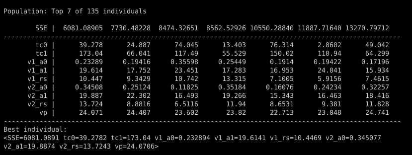
Parameters tc0 and tc1 are the time constants for two IIR lowpass filter stages, mimicking the thermal mass of the temperature sensor. Parameters v1_a0, v1_a1, and v1_rs are the terms for the nonlinear curve for the first thermistor voltage divider, and the three parameters starting with v2_ are the same for the second voltage divider. Finally, parameter vp is the nominal 23V voltage supplied by the Yocto-0-10V-Rx.

The values of tc0 and tc1 are subject to a constraint, which must be satisfied for the individual to even be evaluated and was defined with a keyword of the Population constructor. In this example, the sole constraint is provided by a method of Evaluator that returns True only if the second filter stage has a larger (slower) time constant than the first:

def constraint(self, values):
    """
    Only allows successive time constants that increase with each
    stage. Avoids duplicate evaluation of equivalent filters.
    """
    tcs = [values[x] for x in sorted(values.keys()) if x.startswith('tc')]
    return np.all(np.greater(np.diff(tcs), 0))

This keeps ade from having to consider combinations of filter stages that are exactly equivalent, cutting the search space in half. You can use constraints to rule out bogus, duplicative, or doomed combinations of parameters and do the hard work of evaluation only on unique and viable individuals.

Now, the best individuals randomly chosen for the initial population in this example don’t look too promising. The very best one has a sum-of-squared-error (SSE) of about 6,000, and things fall off rapidly after that. Let’s watch how quickly a little evolution improves on pure randomness.¹²

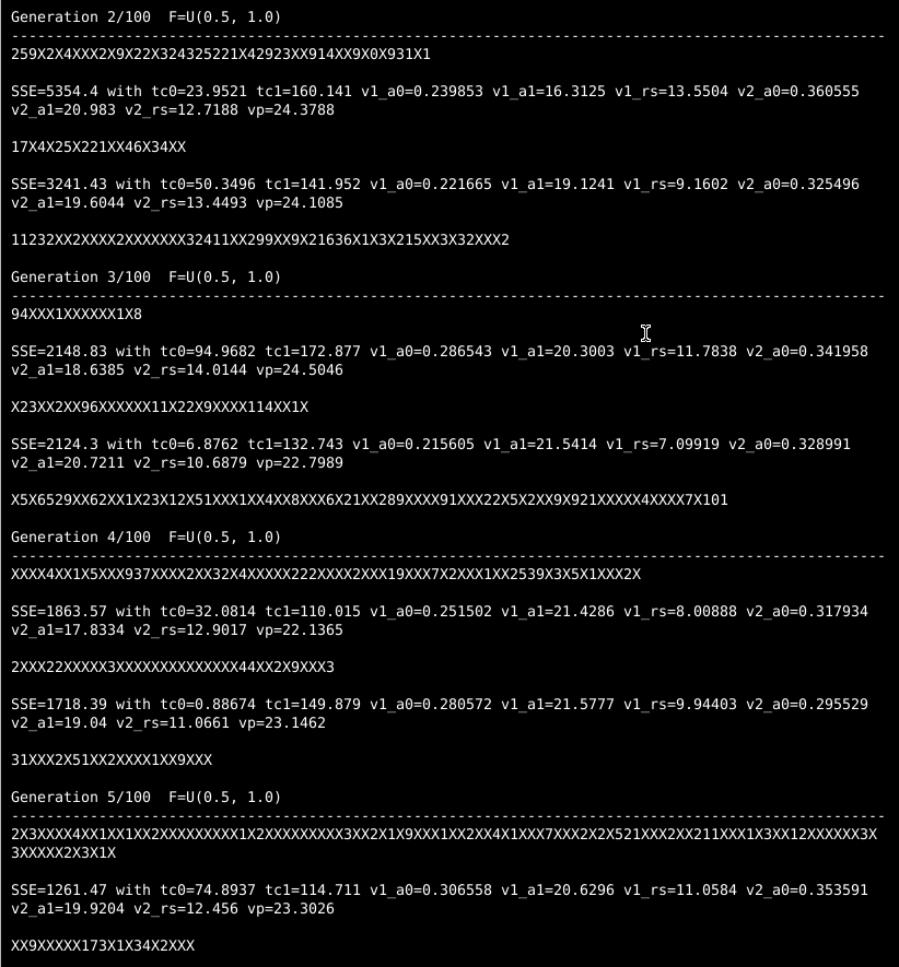
Midway through the second generation, differential evolution has found a successful challenger with half the SSE of the best initial individual!¹³ And by the fifth generation, the best challenger has an SSE not even half as bad as that.

You can see the outcome of each tournament between target and its challenger with the characters that march across the console while ade is running in your terminal. If the character is an “X”, the challenger was worse and the target keeps its place. If the character is a numeric digit, the challenger won its tournament, and the number represents how much better the challenger was than the target it replaced. Early on, there will be a lot of impressive gains as awful randomly-chosen individuals and their early offspring get the boot.

In later generations, most of the characters will be “X” as very good targets demand even better challengers to replace them. And when they do get replaced, the digits mostly will be “1”, which indicates that the challenger was less than 150% better than its target. It’s still progress, but slower. There will also be less frequent reports of a new overall best individual. Take a look at what happened in generation 40, for example:

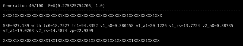
One successful challenger became the overall best individual, with an impressively low SSE of 927. There were only 14 or so other success stories (about 10% of the population), none of which broke the best-individual record, and only one of which had an SSE less than half of the target it replaced. One of the successful challengers was so marginal in its improvement that it got a “0” digit, indicating that it was less than 1% better than the target it replaced.

Something else is different in generation 40: The lower bound for the F differential scaling factor is no longer 0.5. The default behavior of ade is to automatically adjust F with each generation once improvements slow down. First it reduces the lower bound of F, then the upper bound, when the challengers’ improvements aren’t quite adding up anymore.

Eventually, when the range for randomly choosing a value of F becomes so small and low that the optimization is just tweaking around a local minimum, ade stops and reports its final result. In this example, that happened after 70 generations, with a result that was only about 1.5% better than the one that showed up in generation 40, and about 5% better than the result found in generation 20.

You can wait for minor improvements as long as you want (see the bitterEnd option to the DifferentialEvolution constructor), but don’t feel bad about seeing slow progress after a certain point. Most of your own DNA evolution got done in single-celled organisms a billion years ago. A newborn baby adopted from your ancestors 20,000 years ago could grow up and go to college, graduate just fine, and not look or act out of place.

License

Copyright (C) 2017-2018 by Edwin A. Suominen, http://edsuom.com/:

See edsuom.com for API documentation as well as information about
Ed's background and other projects, software and otherwise.

Licensed under the Apache License, Version 2.0 (the "License");
you may not use this file except in compliance with the
License. You may obtain a copy of the License at

  http://www.apache.org/licenses/LICENSE-2.0

Unless required by applicable law or agreed to in writing,
software distributed under the License is distributed on an "AS
IS" BASIS, WITHOUT WARRANTIES OR CONDITIONS OF ANY KIND, either
express or implied. See the License for the specific language
governing permissions and limitations under the License.

Notes